7.3 Version NERPMAB2
7.3 VERSION NERPM-AB2
This section documents the set of improvements that were made to the NERPM model for the release of NERPM-AB2. The improvements focused on:
- Base year updated from 2010 to 2015
- Re-built all land use inputs for 2015 and future
- Switched from parcels to microzones to ease data preparation
- Switched from PopGen to PopulationSim
- Updated the highway network to 2015 (NFTPO)
- Updated the transit network to 2016 (JTA)
- Updated external traffic volumes and distributions based on Bluetooth OD data (FDOT)
- Upgraded from the NFTPO specific version of DaySim to the multiple-agency (a.k.a. core) version, which is faster, more stable, and includes new features such as Transportation Network Companies (TNC) mode (i.e. Uber and Lyft)
- Updated future year scenarios
Contents
- 1 Parcel to Microzone (MAZ)
- 2 Land-use data updated to base year 2015
- 3 PopulationSim
- 4 Development of 2045 land-use data
- 5 Development of 2045 control data
- 6 Updating 2045 control data
- 7 Development of 2030 land-use data
- 8 Development of 2030 control data
- 9 Updating 2030 control data
- 10 DaySim ABM Model Update
- 10.1 Table: Estimated Households by Number of Vehicles and County (Parcel)
- 10.2 Table: Estimated Households by Number of Vehicles and County (Microzone + Node to Node Distances)
- 10.3 Table: Estimated Households by Number of Vehicles and County (Microzone + N2N Distances + PopSim 2015)
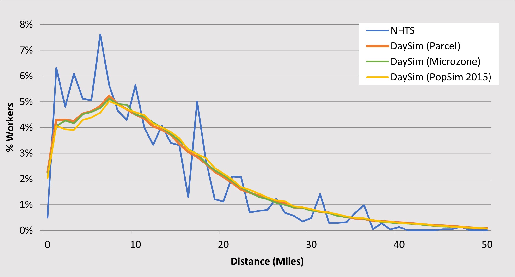
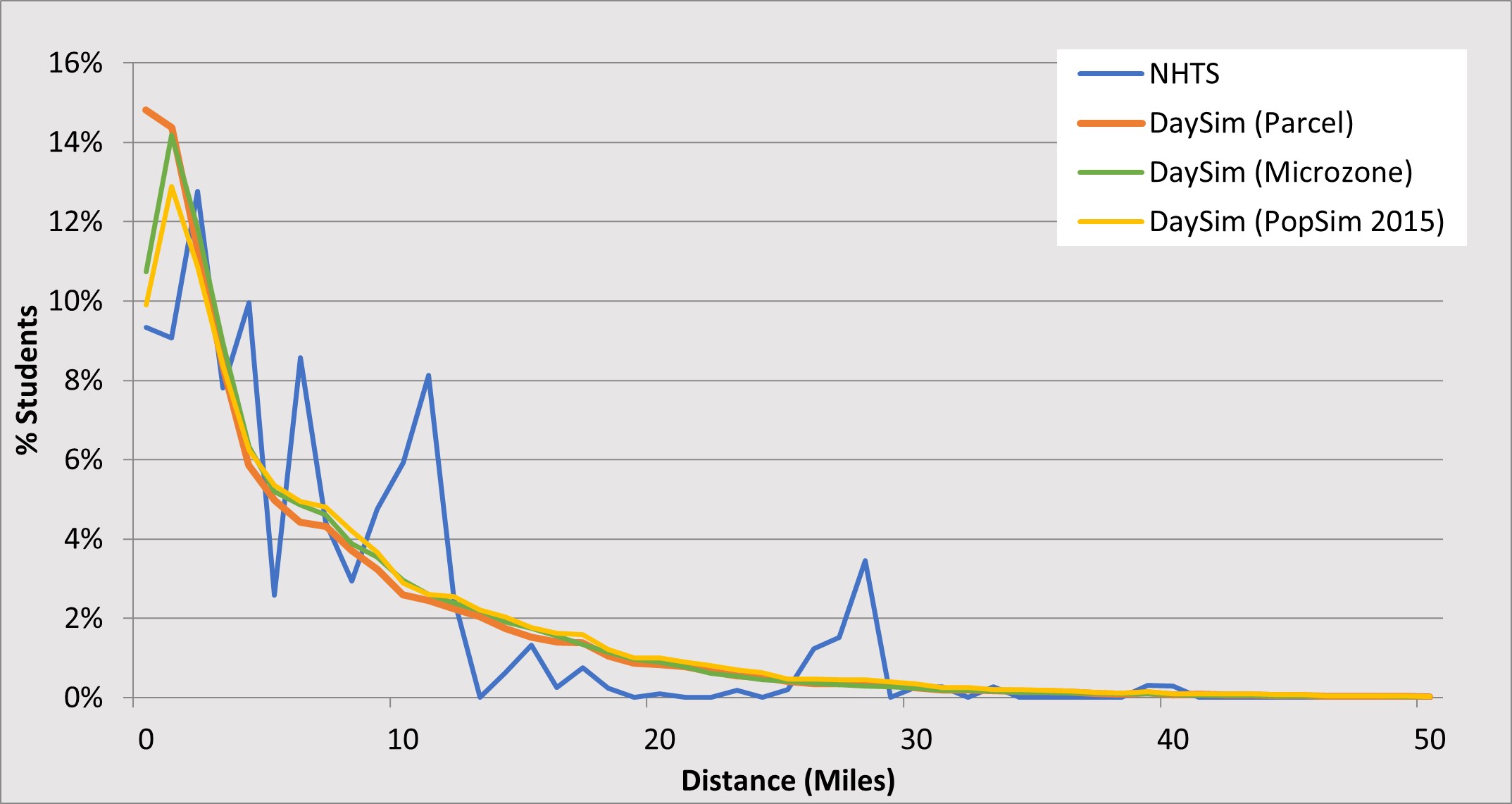
- 10.4 Work Location Choice: HOME-WORK DISTANCES
- 10.5 School Location Choice: HOME-SCHOOL DISTANCES
- 11 Development of External Model Inputs
- 12 Network Updates
- 13 CUBE Model Update
- 14 DaySim Model Calibration and Validation
- 15 Model Calibration and Validation
- 16 Software Requirements
- 17 Setup and Run PopulationSim
- 18 Preparing DaySim Inputs
- 19 DaySim Data Editing
Parcel to Microzone (MAZ)
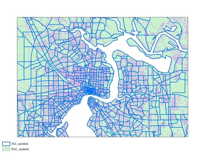
In the previous version of the model, the unit of spatial analysis was parcels. There were approximately 700,000 parcels in the region, which made it difficult to maintain, edit and attribute, both the existing and alternative scenarios. This led to the creation and use of microzones as an alternative, which is halfway between parcels and TAZs and are easier to maintain. As you can see in the table, there are around 55 thousand microzones against 700 thousand parcels. This makes it much easier for the user to update land use information such as employment, enrollment etc. The total number of TAZs in this version is 1862. The plot shows the TAZ and the MAZ layer around downtown Jacksonville. This shows how TAZs and MAZs are related. You can see in the plot that MAZs in downtown tend to be smaller than the ones in the periphery. If you have any questions about the development of MAZs, please refer to the model documentation for more details.
| County |
Number of Parcels |
% Freq |
Number of MAZ |
% Freq |
Number of TAZ |
% Freq |
|---|---|---|---|---|---|---|
| Baker |
12,490 |
1.78 |
1,735 |
3.14 |
29 |
1.56 |
| Clay |
84,529 |
12.02 |
7,796 |
14.13 |
184 |
9.88 |
| Duval |
355,805 |
50.59 |
28,263 |
51.22 |
1,281 |
68.80 |
| Nassau |
47,443 |
6.75 |
4,455 |
8.07 |
108 |
5.80 |
| Putnam |
102,053 |
14.51 |
6,652 |
12.05 |
44 |
2.36 |
| St. Johns |
100,950 |
14.35 |
6,283 |
11.39 |
216 |
11.60 |
| Total |
703,270 |
100.00 |
55,184 |
100.00 |
1,862 |
100.00 |
Figure: MAZ and TAZ layer in Downtown Jacksonville
Land-use data updated to base year 2015
Once the microzones were formed the following land-use data were updated for the base year 2015:
Household Data
The household data at parcel level was aggregated to microzone level for the base year 2015.
Employment Data
The employment data was updated using three sources of data:
- The 2010 parcel employment data projected to 2015
- Data provided by Infogroup and edited by North Florida TPO
- Data provided by Cambridge Systematics as described in their June 30, 2017 memorandum “Development of 2015 Employment Data” for FDOT
Please refer to the model documentation for the details on how these data sources were utilized.
School Enrollment Data
School enrollment data from the Florida Department of Education (FDOE) provided by North Florida TPO was used to develop school enrollment data at microzone level for the base year 2015. The details of this development process can be found in the model documentation.
Parking
The parking data was derived from Florida DOT parking shapefiles "Parking surface" and "g100freeway". The website Jacksonville, FL Parking was also used along with the shapefiles to develop parking data.
Lodging
A list of 367 known hotels, motels, and bed and breakfasts from the Florida Department of Business and Professional Regulation provided by North Florida TPO was used to develop lodging information.
Special Generators
Jacksonville International Airport and St. Augustine are the two special generators that are effectively acting as a special generators in the model.
The Airport had an attraction value of 15,000 in 2010. Based on several sources, RSG determined that the passenger traffic at the airport has decreased slightly between 2010 and 2015. CAPA – Centre for Aviation noted an overall downward trend in traffic since 2008 but traffic began to pick up in 2013 . The airport’s website lists the 2010 and 2015 number of passengers as 5,602,000 and 5,502,000 respectively, which represents a 1.8% reduction in traffic. FDOT’s 2015 Airport Profile of JAX showed similar findings. Given the small change over the years, we recommend leaving the airport’s attraction value at 15,000 for 2015.
St. Augustine had an attraction value of 2,288 in 2010. This number accounts for tourists coming to the area. In 2010 and 2015, St. Johns County had 3.4 million and 6.3 million visitors, respectively, which represents an 85% growth over the five-year period. The 2015 number was considered an anomaly because it was the City’s 450th birthday. However, 2016 was even higher with 6.8 million visitors, so an 85% increase may be reasonable. Increasing the attractions value by 85% to 4,240 could have a noticeable impact on links near the TAZ.
PopulationSim
- PopulationSim is an open platform for population synthesis
- Replaced PopGen in this version of NERPM-AB
- Has better demographic and geographic methods compared to PopGen
- Actively maintained by the travel modeling community
- Run only when there are major changes in the landuse data
Input Data
The main inputs to a population synthesizer are
- Disaggregate population samples (Seed Sample)
- Marginal control distributions (Control variables)
The Seed sample is obtained from the Census Public Use Microdata Sample (PUMS) and the Marginal distributions of person and household attributes are obtained from Bureau of Economic and Business Research (BEBR) and Census respectively.
The next step is the preparation of inputs to PopulationSim which includes:
Geographic cross-walk
PopulationSim can handle any number of nested geographies. The geography level (hierarchy) selected for NERPM-AB 2015 to which the marginal distributions are specified are as follows:
- Meta Geography: Super County (SCOUNTY)
- Seed Geography: PUMA
- Sub-seed Geography: TAZ and MAZ
Super-County is chosen instead of County due to overlapping of county and PUMA boundaries. Super County is the combination of multiple County to form one geographic area.
Seed population (Household and Person tables)
One of the main requirements for the seed sample is that it should be representative of the modeling region. The seed sample is obtained from PUMS dataset. The PUMS data contain five years of household records. The seed sample should be representative of the modeling region. It must contain all the specified control variables, as well as any variables that are needed for the travel model but not specified as controls. The PUMS data is downloaded from PUMS website and it is extracted both demographically and geographically for the North Florida TPO region using PUMA codes conforming to the region. There are 11 PUMA regions in the North Florida TPO area. The seed sample must include an initial weight field. The model setup includes the Seed sample that contains a weight field, WGTP, which is used for control of total households.
Controls
Controls or targets are the marginal distributions that form the constraints for the population synthesis procedure. The objective of the population synthesis procedure is to produce a synthetic population with attributes matching these marginal distributions. The controls were developed at three geographic levels:
Super County
The raw input data was downloaded at county level from BEBR. Next, the data was aggregated to super county level. The data at super county level are person level attributes:
- Male
- Female
- Age 0-4
- Age 5-17
- Age 18-24
- Age 25-54
- Age 55+
Table: BEBR Super County Totals (2015)
| SCOUNTY | PERSONS | MALE | FEMALE | AGE0-4 | AGE5-17 | AGE18-24 | AGE25-54 | AGE55+ |
|---|---|---|---|---|---|---|---|---|
| 12109107 | 286,322 | 140,049 | 146,273 | 15,257 | 47,539 | 23,702 | 104,701 | 95,123 |
| 12031000 | 905,574 | 440,059 | 465,515 | 61,304 | 146,443 | 87,517 | 379,741 | 230,569 |
| 12003089 | 103,553 | 51,969 | 51,584 | 5,963 | 16,366 | 8,505 | 38,968 | 33,751 |
| 12019000 | 201,277 | 98,400 | 102,877 | 12,543 | 37,662 | 18,453 | 79,447 | 53,172 |
TAZ
The raw input data was downloaded at various levels [Source: 2011-15 American Community Survey five-year estimates, ACS5] and it was processed at TAZ level to generate household attributes:
- Households by Household Size at Block Group Level
- Household Size 1
- Household Size 2
- Household Size 3
- Household Size 4+
- Tenure by Age of Householder at Block Group Level
- Householder Age 15-44
- Householder Age 45-64
- Householder Age 65+
- Households by number of workers at Census Tract Level
- Zero household workers
- One household workers
- Two household workers
- Three or more than three household workers
- HHs by income at Census Tract Level
- Household income $0-$24,999
- Household income $25,000-$59,999
- Household income $60,000-$99,999
- Household income $100,000+
MAZ
The raw input data was obtained at parcel level for the year 2010 and calculated for 2015 using growth factor from 2010 to 2015. The data obtained is total number of households and then aggregated for each MAZ. Once the control files are prepared, the total number of households and persons are calculated across geographies to check for consistency as shown in Table below.
Table: Control data summary (2015)
| Data | Geography | Value |
|---|---|---|
| Total number of households | MAZ | 582,199 |
| Total number of households | TAZ | 582,199 |
| Number of households in HHSIZE=1 | TAZ | 155,522 |
| Number of households in HHSIZE=2 | TAZ | 196,050 |
| Number of households in HHSIZE=3 | TAZ | 87,996 |
| Number of households in HHSIZE=4+ | TAZ | 110,821 |
| Total number of persons (from HHSIZE) | TAZ | 1,397,535 |
| Total number of persons | SCOUNTY | 1,397,534 |
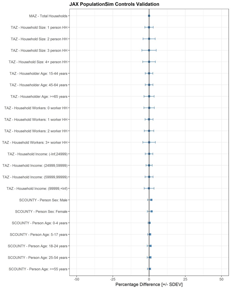
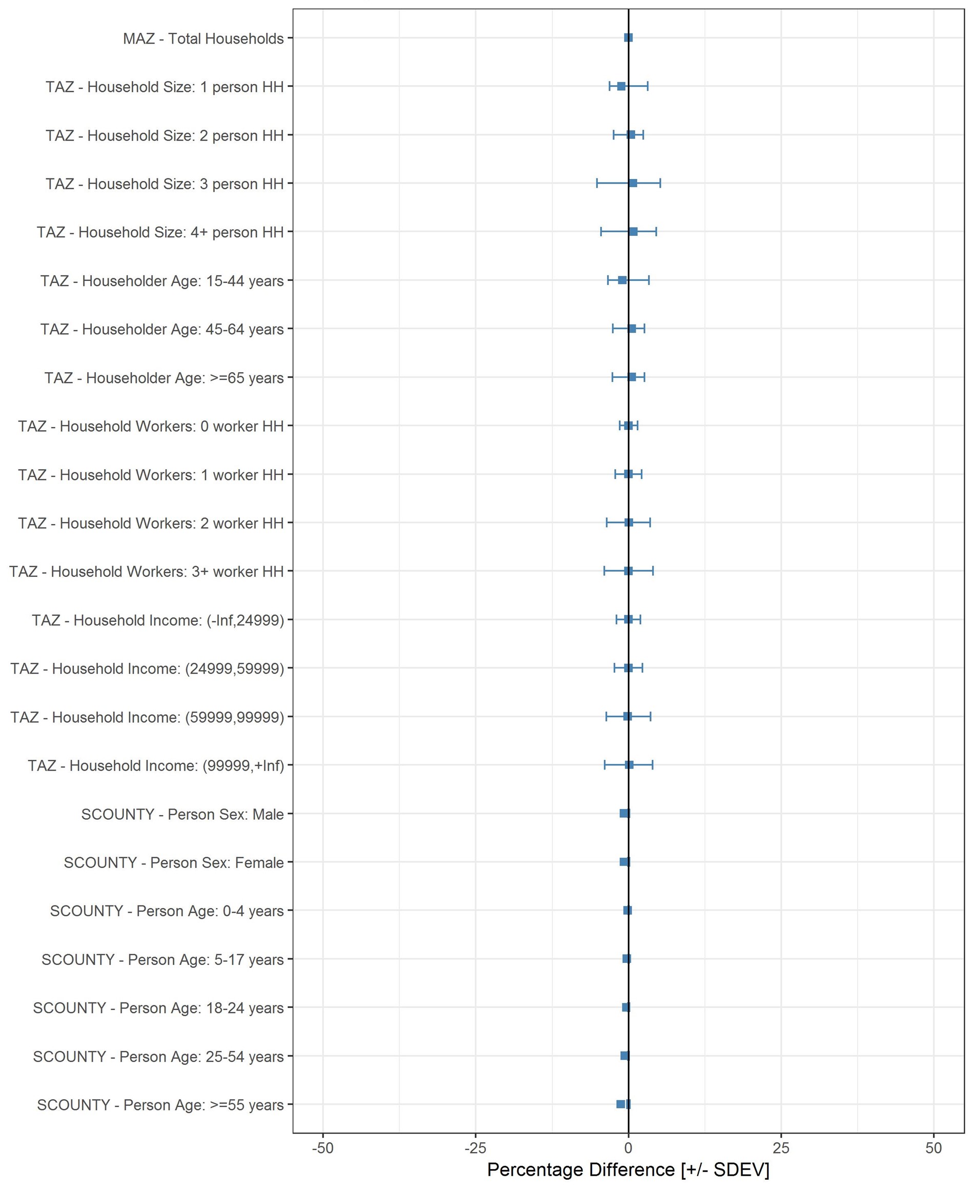
In this figure, we see the performance of PopulationSim as it tries to match the controls. In this version of the model, controls such as household size, householder age, household income etc. were used at different levels of geography. The standard deviation (STDEV) of the percentage difference informs us of how much dispersion from the average exists. As you can see, the total number of households at the MAZ level matches perfectly with the controls. PopulationSim does that by design. And we see a very close match on all the other controls as well.
Development of 2045 land-use data
The 2045 land-use data was created by applying a methodology, detailed in the model documentation, to the land-use data for the base year (2015) and the BEBR forecasts. The table below shows the summary of comparisons between land-use data for the base year (2015) and the future year (2045).
Table: Comparison of 2015 and 2045 totals
| COUNTY | Households 2015 |
Households 2045 |
Employment 2015 |
Employment 2045 |
Enrollment 2015 |
Enrollment 2045 |
|---|---|---|---|---|---|---|
| NASSAU | 32,983 | 51,902 | 28,480 | 55,393 | 13,368 | 31,576 |
| DUVAL | 357,463 | 541,730 | 496,394 | 708,478 | 211,091 | 362,983 |
| ST JOHNS | 84,540 | 181,500 | 66,355 | 179,066 | 43,977 | 116,687 |
| CLAY | 70,523 | 132,830 | 46,539 | 105,158 | 40,877 | 98,998 |
| BAKER | 8,815 | 15,117 | 8,909 | 18,491 | 5,128 | 9,876 |
| PUTNAM | 31,278 | 40,307 | 21,521 | 35,564 | 14,856 | 23,404 |
| TOTAL | 585,602 | 963,386 | 668,198 | 1,102,150 | 329,297 | 643,524 |
Development of 2045 control data
Controls at three levels of geography are required to run PopulationSim for North Florida TPO: Super County, TAZ and MAZ. The Super COUNTY level controls were obtained from BEBR data and the TAZ and MAZ level controls were prepared using the 2045 land-use data. Please refer to the model documentation for the details of this development process.
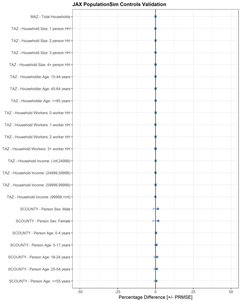
In this figure, we see the performance of PopulationSim as it tries to match the controls. In this version of the model, controls such as household size, householder age, household income etc. were used at different levels of geography. The standard deviation (STDEV) of the percentage difference informs us of how much dispersion from the average exists. As you can see, the total number of households at the MAZ level matches perfectly with the controls. PopulationSim does that by design. And we see a very close match on all the other controls as well.
Updating 2045 control data
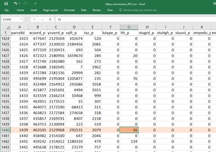
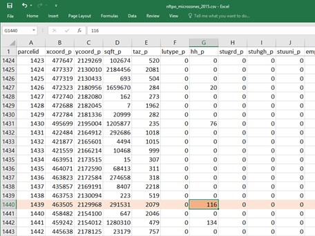
When updating land-use data it is necessary to update the PopulationSim controls. The following example shows how to update the controls when adding 100 households to MAZ 1439:
Land-use file before update
- Update the land-use “nftpo_microzones_2045.csv” file by adding 100 households to MAZ 1439. The figure above shows the land-use file before the addition of 100 households and the figure below shows the land use file after the addition of 100 households.
Land-use file after update
- Edit the variables listed in the table below within the CUBE script “update_controls.S” located in “./User.prg/Population_Synthesis/” folder. The script performs following actions:
- Makes a copy of control files.
- Updates MAZ level household controls by comparing existing control values with land-use values.
- Updates TAZ level household controls by aggregating land-use values by TAZ. Redistributes the additional households by household size based on the distribution of households by household size as observed in control data. Similarly redistributes additional household based on distribution of households by householder age, number of household workers, and household income respectively as observed in the control data.
- Updates County level population controls by adding additional person based on average household size calculated for each county from existing controls. The additional population is distributed across gender and age group based on distribution of population observed in controls for respective categories.
Table: Variables to update by user when updating update_control.S script
| VARIABLE NAME | DESCRIPTION | EXAMPLE |
|---|---|---|
| LANDUSE_PATH | Full path to the folder that contains the land-use file. | 'E:\NERPMABv2.0\User.prg\DaySim_Data_Tools' |
| LANDUSE_FILE | Name of the land-use file | 'nftpo_microzones_2045.csv' |
| POPSIM_PATH | Full path to the PopulationSim folder | 'E:\NERPMABv2.0\User.prg\Population_Synthesis' |
| CONTROL_FOLDER | Name of the folder containing the control data | 'data_2045' |
| OVERWRITE_INITIAL | A value of 0 will not overwrite the initial files and a value of 1 will overwrite the initial files. | 0: Does not overwrite the control_totals_{zone}_initial.csv file 1: Overwrites the control_totals_{zone}_initial.csv file |
- Run “update_controls.bat” file, located in “./User.prg/Population_Synthesis/” folder, by double-clicking. This will call the Cube Voyager and run the “update_controls.S” script.
- The control files are now updated and are ready to be used by PopulationSim.
Development of 2030 land-use data
The 2030 land-use data was created by applying a methodology, detailed in the model documentation, to the land-use data for the base year (2015) and the BEBR forecasts. The table below shows the summary of comparisons between land-use data for the base year (2015) and the future year (2030).
Table: Comparison of 2015 and 2030 totals
| COUNTY | Households 2015 |
Households 2030 |
Employment 2015 |
Employment 2030 |
Enrollment 2015 |
Enrollment 2030 |
|---|---|---|---|---|---|---|
| NASSAU | 32,983 | 41,948 | 28,480 | 45,394 | 13,368 | 25,998 |
| DUVAL | 357,463 | 453,184 | 496,394 | 622,922 | 211,091 | 311,765 |
| ST JOHNS | 84,540 | 135,295 | 66,355 | 124,742 | 43,977 | 79,721 |
| CLAY | 70,523 | 100,980 | 46,539 | 81,119 | 40,877 | 75,838 |
| BAKER | 8,815 | 12,212 | 8,909 | 14,615 | 5,128 | 7,602 |
| PUTNAM | 31,278 | 35,535 | 21,521 | 32,993 | 14,856 | 22,076 |
| TOTAL | 585,602 | 779,154 | 668,198 | 921,785 | 329,297 | 523,000 |
Development of 2030 control data
Controls at three levels of geography are required to run PopulationSim for North Florida TPO: Super County, TAZ and MAZ. The Super COUNTY level controls were obtained from BEBR data and the TAZ and MAZ level controls were prepared using the 2030 land-use data. Please refer to the model documentation for the details of this development process.
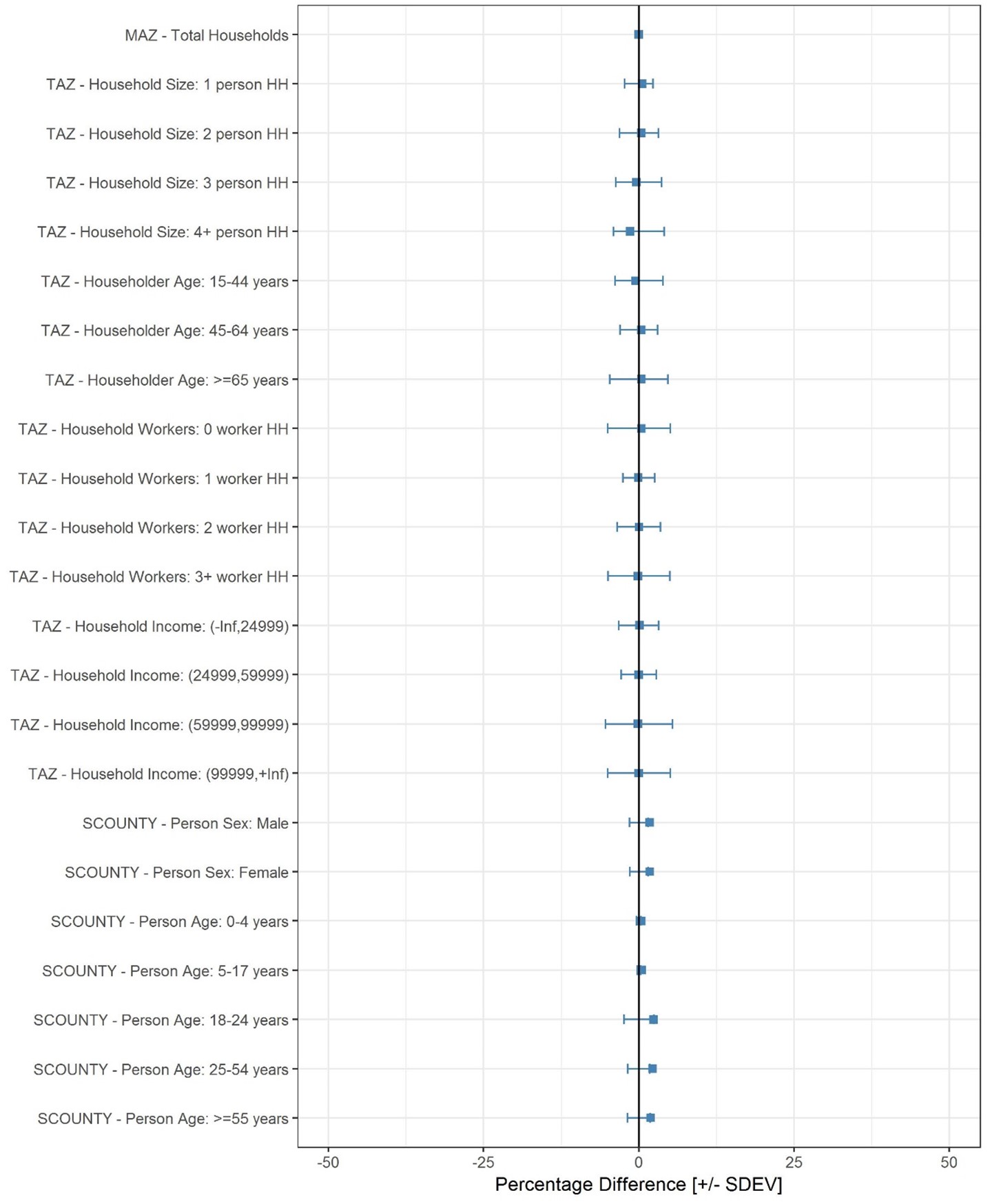
In this figure, we see the performance of PopulationSim as it tries to match the controls. In this version of the model, controls such as household size, householder age, household income etc. were used at different levels of geography. The standard deviation (STDEV) of the percentage difference informs us of how much dispersion from the average exists. As you can see, the total number of households at the MAZ level matches perfectly with the controls. PopulationSim does that by design. And we see a very close match on all the other controls as well.
Updating 2030 control data
When updating land-use data it is necessary to update the PopulationSim controls. The following example shows how to update the controls when adding 100 households to MAZ 1439:
Land-use file before update
- Update the land-use “nftpo_microzones_2045.csv” file by adding 100 households to MAZ 1439. The figure above shows the land-use file before the addition of 100 households and the figure below shows the land use file after the addition of 100 households.
Land-use file after update
- Edit the variables listed in the table below within the CUBE script “update_controls.S” located in “./User.prg/Population_Synthesis/” folder. The script performs following actions:
- Makes a copy of control files.
- Updates MAZ level household controls by comparing existing control values with land-use values.
- Updates TAZ level household controls by aggregating land-use values by TAZ. Redistributes the additional households by household size based on the distribution of households by household size as observed in control data. Similarly redistributes additional household based on distribution of households by householder age, number of household workers, and household income respectively as observed in the control data.
- Updates County level population controls by adding additional person based on average household size calculated for each county from existing controls. The additional population is distributed across gender and age group based on distribution of population observed in controls for respective categories.
Table: Variables to update by user when updating update_control.S script
| VARIABLE NAME | DESCRIPTION | EXAMPLE |
|---|---|---|
| LANDUSE_PATH | Full path to the folder that contains the land-use file. | 'E:\NERPMABv2.0\User.prg\DaySim_Data_Tools' |
| LANDUSE_FILE | Name of the land-use file | 'nftpo_microzones_2030.csv' |
| POPSIM_PATH | Full path to the PopulationSim folder | 'E:\NERPMABv2.0\User.prg\Population_Synthesis' |
| CONTROL_FOLDER | Name of the folder containing the control data | 'data_2030' |
| OVERWRITE_INITIAL | A value of 0 will not overwrite the initial files and a value of 1 will overwrite the initial files. | 0: Does not overwrite the control_totals_{zone}_initial.csv file 1: Overwrites the control_totals_{zone}_initial.csv file |
- Run “update_controls.bat” file, located in “./User.prg/Population_Synthesis/” folder, by double-clicking. This will call the Cube Voyager and run the “update_controls.S” script.
- The control files are now updated and are ready to be used by PopulationSim.
DaySim ABM Model Update
After completion of base year 2015 data aggregation from parcels to microzones, DaySim was tested for the new geographies and the results compared against the parcel results to check for consistencies. The necessary input files were created for DaySim run as explained in detail in Appendix B of the model documentation. After a successful run of DaySim using updated 2015 Microzone and Population synthesis dataset, the results were compared with previous DaySim run using parcels. The small set of tables and figures displayed here show the consistency of the 2015 dataset in DaySim performance. A complete series of tables and figures are shown in the model documentation.
Table: Estimated Households by Number of Vehicles and County (Parcel)
| County | Number of Vehicles | ||||||
|---|---|---|---|---|---|---|---|
| 0 | 1 | 2 | 3 | 4+ | Total | % Total | |
| Baker | 309 | 2,750 | 3,899 | 1,285 | 557 | 8,800 | 2% |
| Clay | 2,154 | 19,501 | 32,064 | 11,436 | 4,123 | 69,278 | 12% |
| Duval | 27,194 | 126,487 | 137,367 | 42,231 | 15,633 | 348,912 | 61% |
| Nassau | 1,212 | 10,006 | 14,514 | 4,681 | 1,820 | 32,233 | 6% |
| Putnam | 1,594 | 11,944 | 12,800 | 3,767 | 1,543 | 31,648 | 6% |
| St. Johns | 3,097 | 25,256 | 36,209 | 11,566 | 4,102 | 80,230 | 14% |
| Total | 35,560 | 195,944 | 236,853 | 74,966 | 27,778 | 571,101 | 100% |
Table: Estimated Households by Number of Vehicles and County (Microzone + Node to Node Distances)
| County | Number of Vehicles | ||||||
|---|---|---|---|---|---|---|---|
| 0 | 1 | 2 | 3 | 4+ | Total | % Total | |
| Baker | 333 | 2,781 | 3,868 | 1,261 | 557 | 8,800 | 2% |
| Clay | 2,491 | 19,945 | 31,772 | 11,122 | 3,948 | 69,278 | 12% |
| Duval | 28,867 | 126,963 | 136,315 | 41,659 | 15,108 | 348,912 | 61% |
| Nassau | 1,329 | 10,195 | 14,426 | 4,515 | 1,768 | 32,233 | 6% |
| Putnam | 1,627 | 11,994 | 12,767 | 3,750 | 1,510 | 31,648 | 6% |
| St. Johns | 3,795 | 25,835 | 35,721 | 11,105 | 3,774 | 80,230 | 14% |
| Total | 38,442 | 197,713 | 234,869 | 73,412 | 26,665 | 571,101 | 100% |
Table: Estimated Households by Number of Vehicles and County (Microzone + N2N Distances + PopSim 2015)
| County | Number of Vehicles | ||||||
|---|---|---|---|---|---|---|---|
| 0 | 1 | 2 | 3 | 4+ | Total | % Total | |
| Baker | 403 | 3,021 | 3,704 | 1,015 | 672 | 8,815 | 2% |
| Clay | 2,742 | 21,083 | 31,758 | 11,032 | 3,908 | 70,523 | 12% |
| Duval | 29,793 | 131,763 | 131,610 | 44,856 | 16,038 | 354,060 | 61% |
| Nassau | 1,471 | 12,051 | 13,617 | 3,469 | 2,375 | 32,983 | 6% |
| Putnam | 2,158 | 13,690 | 10,852 | 3,059 | 1,519 | 31,278 | 5% |
| St. Johns | 3,652 | 28,418 | 37,278 | 11,588 | 3,604 | 84,540 | 15% |
| Total | 40,219 | 210,026 | 228,819 | 75,019 | 28,116 | 582,199 | 100% |
Work Location Choice: HOME-WORK DISTANCES
School Location Choice: HOME-SCHOOL DISTANCES
Development of External Model Inputs
Data Sources
The source data for the X-X trip table has been obtained from Bluetooth detectors that were installed at 17 locations adjacent to highways at external model stations. This work was conducted under a separate contract with Florida DOT. The raw data from the Bluetooth deployment were obtained by HNTB and processed for further analysis by RSG.
- 2010 North Florida TPO model X-X trip table (EETRIPS.dbf): (29 nodes)
The total trips originating for each external node and destined for other external nodes are calculated by assigning a proportion of the total incoming traffic (e.g. 16%). Incoming traffic is distributed from each origin external node to each other external node in proportion to the destination node’s AADT.
- EE_O-D_Study spreadsheet provided by HNTB: (17 nodes)
This spreadsheet was provided by HNTB and contains the raw matched BT X-X data, total traffic counts, total truck counts, matched BT X-X/X-I data (17 external and 150 internal nodes), and related pivot tables.
Estimating the BT Expansion Factor
The BT expansion factor (or penetration rate) is the percentage of total traffic recorded with having a discoverable Bluetooth device on or within the vehicle. The expansion factors imputed from the HNTB data were abnormally high given RSG’s prior experience in working with data of this type. RSG requested, but never received from HNTB, the raw Bluetooth data. For this reason, RSG developed a method to estimate an expansion factor for each station. The details of the method can be found in the model documentation.
Estimating External-External Trips
The raw matched X-X BT data alongside with expansion factors are used to estimate the X-X trips. The data is cleaned based on methodology described in the model documentation.
Network Updates
Network Link Updates
The previous Existing + Committed (E+C) network, known as 2040A in the 2010 model setup, was used as the starting point for the 2015 network. Table below lists the previous E+C network links that were modified to be consistent with 2015 base year conditions. Modifications included revisions to the number of lanes, facility type, and turn restrictions.
UPDATE (01/30/2020): BUSTFAC_45C was set to 0 in the 2045 network fields. This was causing problems with transit assignment resulting in very low transit ridership. RSG set this to 1 for all links since BUSTFAC_15A has it set to 1 for all links. This resolved the low transit ridership issue in the scenario year 2045.
Before setting up a model run, please make sure that in the transit route input file (or any subsequent transit route input files), the skyway modes are coded as MODE equal 24 instead of 23 and commuter rail “CR_SE-Rail” is coded as MODE equal 25 instead of 27 to be consistent with the new in-vehicle time skims.
E+C Network (2040A) Links to Change for 2015 Network
| County | Route | From | To |
|---|---|---|---|
| Nassau | Chester Rd. | SR A1A | Green Pine Rd. |
| Duval | First Coast Expwy. (SR 23) | Clay CL | Argyle Forest Blvd. |
| Duval | First Coast Expwy. (SR 23) | Argyle Forest Blvd | I-10 |
| Clay | First Coast Expwy. (SR 23) | Blanding Blvd (SR 21) | Duval CL |
| Duval | I-10 @ I-95 | Roosevelt Ave. (US 17) | San Marco Ave. |
| Duval | I-295 | SR 9B | J.T. Butler Blvd. (SR 202) |
| Duval | I-295 | I-10 | Commonwealth Ave. |
| Duval | I-295 | Buckman Bridge | I-95 |
| Duval | I-295 | I-95 (South) | SR 9B |
| Duval | Martin Luther King Jr. Pkwy | at 21st St./Talleyrand Ave. | |
| Duval | SR 9B | Philips Hwy. (US1) | I-295 |
| Duval | SR 9B | I-95 | Philips Hwy. (US1) |
| Duval | US 301 (SR 200) | South of Baldwin | North of Baldwin |
| Duval | Blanding Blvd/SR 21 | South of Old Jennings | North of CR 218 |
| Duval | I-10 @ Beaver Street | Remove access to Beaver Street | |
| Nassau | US 301 (SR 200) | Duval CL | Callahan |
Volume Count Updates
The North Florida TPO provided AADT counts from 2015 FDOT portable traffic monitoring sites at point locations throughout the network. Each count was for total vehicles and did not include directionality or time of day factors. It was assumed that counts on bidirectional roads were equally split between both directions.
These points were spatially joined to the network links and then spot checked to ensure the join was accurate. Particular attention was paid to on and off ramps as they tended to have the least accuracy.
The NERPM-AB has four time periods: AM, midday (MD), PM, and night (NT). The 2010 network contains count data for each of these periods on some links. To create time of day count data for the 2015 counts, the 2015 count was distributed between the four time periods using the same ratio as the 2010 counts. Links with a 2015 count but no 2010 time of day counts used nearby 2010 time of day counts. If no 2010 count was nearby, that 2015 count was not used.
CUBE Model Update
Several updates were made to the NERPM-AB Cube model during this project. The previous version of the model had model steps and scripting logic that was left over from the previous four-step model. Therefore, enhancements were made wherever necessary to make sure that the model system and results appear reasonable.
External-Internal Trips Calibration
While looking at auxiliary model demand it was found that IE trips are very long – average VMT per trip is approximately 32 miles, compared to 8 miles for internal trips. The VMT needed to be reduced by factoring either or both total IE or truck trips, or by factoring the length of IE trips for which the gravity model used to distribute them needed adjustment. To help inform this decision, the relationship between the observed counts and the estimated link volumes at external stations was investigated. It was found that both ends of I-95 and on I-10 were low, IE trips needed to be increased. It was also possible that the IE trips were traveling too far, which could be adjusted by making the friction factor curve used in trip distribution for IE trips steeper. A series of steps were taken to resolve this issue as discussed in the model documentation.
Transit Skimming Updates
From the initial transit assignment results, it was found that the skyway/monorail boardings were significantly lower than observed boardings. Therefore, the next model enhancement made was to add alternative-specific constants (ASC) to DaySim for transit modes based on an in-vehicle time skim. For the transit alternatives that need to be modeled in the scenarios, the in-vehicle time (IVT) needs to be skimmed in a separate skim matrix, and any tour or trip that has the transit mode in the OD Pair should get the constant. The updates are discussed in detail in the model documentation.
Highway Skimming for Tolls
In the E+C 2045 networks, express lanes or managed lanes were introduced in the highway network. Initially the toll variable, CARTOLL, was set at zero for all links. This was changed to 20 cents per mile (0.20). This value (CARTOLL) was then multiplied with the link length throughout the model setup to calculate the cost. Moreover, the occupancy for HOV2 and HOV3+ were also changed to 1.3 and 1.5, respectively.
DaySim Model Calibration and Validation
The tour destination and other sub models were calibrated using the North Florida Household Travel Survey (2017), the transit tours and trips were calibrated using the Transit On-Board Survey (2016) obtained from Transit On-Board Survey Program, and the worker flow were calibrated using CTPP (2010) obtained from Census.
The following set of tables and figures show calibration summaries:
Table: Population by Person Type
| Person type | Survey | PopSim |
|---|---|---|
| Full Time Worker | 540,570 | 566,852 |
| Part Time Worker | 96,726 | 59,179 |
| Retired | 172,447 | 142,992 |
| Non-Worker | 203,794 | 208,490 |
| University Student | 43,943 | 55,998 |
| Student Age 16+ | 37,901 | 48,543 |
| Student Age 5-15 | 185,288 | 197,734 |
| Kid under 5 | 83,362 | 102,243 |
| Total | 1,326,484 | 1,419,578 |
Table: Average Home to Work Distance
| Worker Type | Survey | DaySim |
|---|---|---|
| Full Time | 13.7 | 13.3 |
| Part Time | 9.1 | 6.8 |
| Other | 9.9 | 14.5 |
| Total | 13.2 | 12.4 |
Table: Workers by County
| COUNTY | CTPP | HTS | DaySim |
|---|---|---|---|
| 1 | 7,283 | 5,383 | 9,681 |
| 2 | 59,391 | 80,418 | 84,565 |
| 3 | 286,647 | 400,012 | 420,057 |
| 4 | 18,556 | 17,424 | 32,801 |
| 5 | 13,779 | 10,901 | 20,362 |
| 6 | 64,325 | 79,338 | 97,402 |
| TOTAL | 449,980 | 593,476 | 664,868 |
Model Calibration and Validation
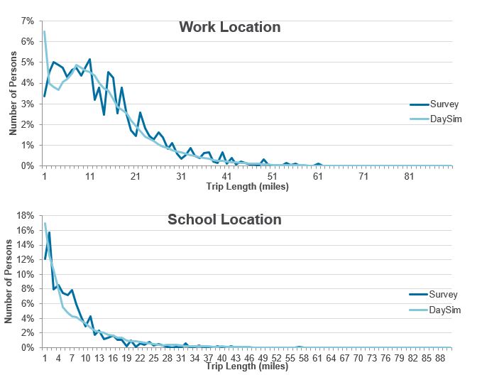
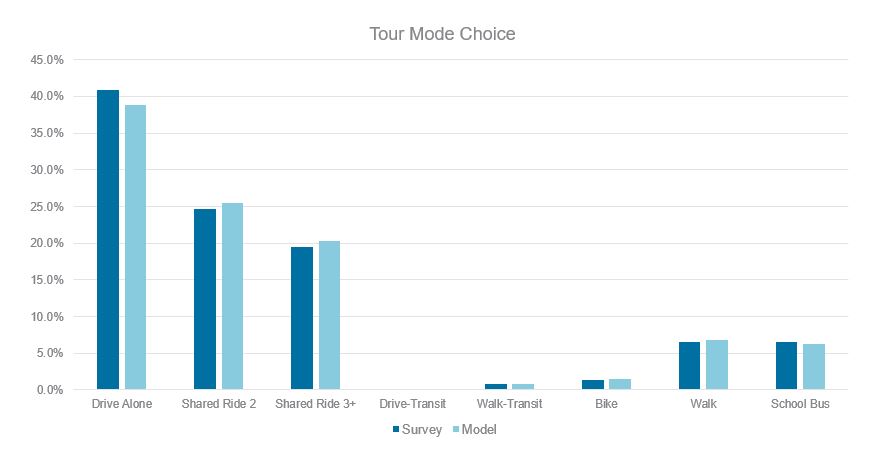
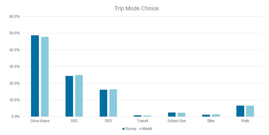
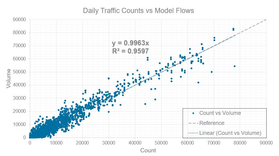
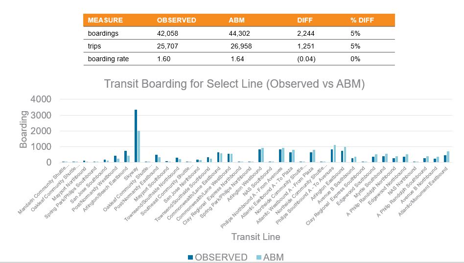
The 2017 north florida travel survey and the 2016 onboard rider demographic survey were used to calibrate the model. Traffic counts and transit boarding counts were used to validate the model outputs. The following tables and figures show the results of the calibrated model. These include trip length frequency distributions, tour and trip mode choice model results, highway and transit validation etc.
Table: Population and Employment
| County | 2015 Population | 2015 Employment | BEA 2015 | 2030 Population | 2030 Employment | 2045 Population | 2045 Employment |
|---|---|---|---|---|---|---|---|
| Baker | 23,138 | 9,649 | 9,695 | 32,340 | 15,876 | 37,723 | 20,123 |
| Clay | 189,600 | 68,871 | 69,317 | 263,882 | 120,166 | 321,984 | 156,073 |
| Duval | 854,757 | 624,952 | 623,596 | 1,078,136 | 786,052 | 1,231,564 | 888,333 |
| Nassau | 76,672 | 30,948 | 31,086 | 97,500 | 49,367 | 116,024 | 60,801 |
| Putnam | 71,687 | 22,605 | 22,780 | 78,328 | 34,695 | 84,790 | 38,102 |
| St Johns | 202,375 | 105,077 | 104,983 | 318,041 | 197,421 | 412,811 | 287,415 |
| Grand Total | 1,418,229 | 862,102 | 861,457 | 1,868,227 | 1,203,577 | 2,204,896 | 1,450,847 |
Trip Length Frequency Distribution
Tour Mode Choice
Trip Mode Choice
Highway Validation
Transit Validation
Software Requirements
PopulationSim requires the following software, already included in the model setup, and can be found in the following location w.r.t the project folder:
- Anaconda2 with Python 2.7 – “.\User.prg\Population_Synthesis\Anaconda2”
Setup and Run PopulationSim
Setup Directory
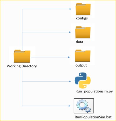
Figure below presents the directory structure for the PopulationSim setup. To set up a PopulationSim run, the user must create the directory structure as shown in below.
PopulationSim Directory Structure
The folders and files in the directory are explained as follows:
- The data directory holds all the input data like seeds data, control data and crosswalks.
- SCOUNTY Control totals
- TAZ Control totals
- MAZ Control totals
- Geographic Crosswalk
- Household Seed table
- Person Seed table
- The Anaconda2 directory houses the core PopulationSim software files and associated libraries and packages.
- The configs folder contains the settings.yaml file and controls.csv file
- PopulationSim is configured using the settings.yaml file. For this project, it is configured to run in base mode which means it is run from beginning to end and produces a new synthetic population
- controls.csv file specifies all the targets, geography, seed table, control field and their expression to the seed table required for the PopulationSim run.
- The output folder will have the final synthetic household and person file and summary attributes after a successful run.
- This batch file activates the PopulationSim environment and then calls the run_populationsim.py Python script to launch a PopulationSim run.
- PopulationSim is run using the RunPopulationSim.bat batch file in Command Prompt Window. Before starting the run, the path to the Anaconda install must be updated within this file.
The PopulationSim procedure is automated and once you have all the data in place, the user just needs to run the batch file from the command prompt window. To run the PopulationSim for 2030 or 2045 the user need to update the ‘data_dir’ field in the settings.yaml file. The ‘data_dir’ field for different scenario years are:
- 2015: The ‘data_dir’ in settings.yaml file should be set to ‘data’
- 2030: The ‘data_dir’ in settings.yaml file should be set to ‘data_2030’
- 2045: The ‘data_dir’ in settings.yaml file should be set to ‘data_2045’
Preparing DaySim Inputs
Transit Files
The transit stops file is created using the input transit network from Jacksonville Transit Authority: TROUTE_{Year}{Alt}.LIN Follow the sequential step below:
- Create a geodatabase (gdb) in Cube
- Import the input transit network file and the highway network file
- Export the nodes (PTNetwork_PTNode) to a shapefile
- Open the shapefile in ArcMap and select the nodes that have STOPNODE=1. These are the transit stops
- Export the selected nodes (stops) to a new stops shapefile. Also Export the transit line file to a shapefile.
- Open the attribute table of the new stops file and add four fields: xcoord_p (double), ycoord_p (double), mode (int) and id (long).
- Calculate xcoord_p and ycoord_p using calculate geometry for the two fields.
- Join transit line by object id and calculate a new field “mode” equal to the MODE field in the line file (1-localbus, 2-skyway). Jacksonville mode codes and daysim mode codes are different, convert these to daysim mode codes before running buffer tools.
| 2015 | 2030 | 2045 | DaySim |
|---|---|---|---|
| 21 = LB | 21 = LB | 21 = LB | 1 = LB |
| 24 = Skyway (coded as LB) | 23 = Skyway (coded as LB) | 23 = Skyway (coded as LB) | 2 = EB |
| 27 = CR | 27 = CR | 3 = CR |
- Calculate stopid as “FID+1”.
- Keep only four fields in the attribute table: id, mode, x_coord, y_coord.
- Export all records in the attribute table to a csv file: nftpo_transitstops.csv
DaySim Data Editing
With the base year moving from 2010 to 2015, microzones replacing parcels and new population data, the inputs for DaySim needed to be updated. The following steps describe the DaySim input data preparation and update for the NERPM-AB model including the tool and input data used and output formed.
Network Data Preparation
This step calculates “nearby” node pairs of microzones for shortest distance path calculations to be used in DaySim.
Tool: Network_DataPrepv2.exe
Directory: \User.prg\DaySim_Data_Tools
Inputs:
- input_node.csv (Node x,ys from an all-streets network)
- jax_MAZs_2015.dat (The coordinates of the newly developed microzones)
- jax_netprep.ctl (Network prep control file)
Output:
- input_od_pairs.csv (for input to shortest path update tool)
Shortest Path Update
This process is required to generate more accurate short distances based on an all streets network. DTALite, a dynamic traffic assignment software, is used to generate node-to-node shortest path distances using the all streets network.
Tool: DTALite64.exe
Directory: \User.prg\DaySim_Data_Tools
Inputs:
- input_od_pairs.csv (from the Network Data Preparation tool)
- input_node.csv (from all-street network)
- input_link_type.csv (from all-street network)
- input_link.csv (from all-street network)
- DTASettings.ini (settings file)
Output:
- output_shortest_path.txt (for input to Buffering microzones)
Buffering micro-zones
The Daysim buffering tool is run to prepare MAZ input file for DaySim. This step calculates the new Microzone buffer measures to be used in DaySim.
Tool: DSBuffTool.exe
Directory: \User.prg\DaySim_Data_Tools
Inputs:
- Jax_microzones_2015.csv (Base Microzone file)
- Jacksonville_Intersections.csv (Street intersections file)
- Jacksonville_transitstops.csv (Transit stops file)
- Jacksonville_openspaces.csv (Open spaces/parks file)
- input_node.csv (All-street Network nodes file)
- output_shortest_path.txt (Node-to-node shortest path distance file)
Output:
- buffered_microzone_2015.dat (to be used in DaySim)
- microzonenode.dat (to be used in DaySim)
- output_shortest_path.txt.bin (Change extension using batch file)
- output_shortest_path.txt.index (Change extension using batch file)
The file extension of the last two outputs above need to be changed for reading into DaySim. The last three output files are used in DaySim to estimate short-distances for car, walk and bike trips.
All three DaySim Data tools can be run using RunAll.bat from the command prompt window.
Running DSBuffTool.exe
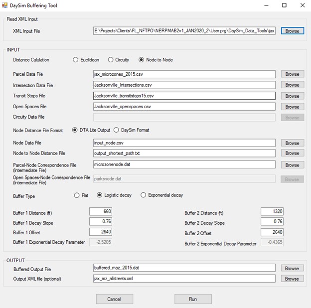
Double-clicking the executable will bring up a GUI as shown in the following figure. The use of this tool is straightforward. The user just needs to specify all the inputs and click on the “Run” button at the bottom of the GUI.
DaySim Buffering Tool GUI
In the “INPUT” section of the GUI, distance calculation and buffer type are set to “Euclidean” and “Logistic decay” respectively. These are the recommended settings for running this tool. If node-to-node distances obtained from an all streets network are available, distance calculation may be set to “Node-to-Node”. The default recommended parameters for logistic decay weights (described in the model design chapter) such as buffer decay slope, offset etc., are also automatically populated in the appropriate fields in the GUI.
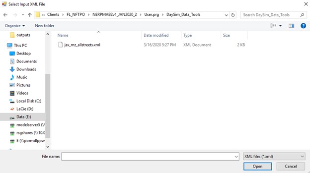
All other inputs are to specify file paths that can be done by clicking on the “Browse” button. This pops a file dialog as show in the figure below. The user may also enter full file paths manually using keyboard.
Buffer Tool File Selection Dialog
All file specification fields for the tool are described below. Details about formats for the input files can be found in the directory and data structures chapter.
- MAZ Data File: This is the base MAZ file. It is obtained by running the disaggregation tool.
- Intersection Data File: This file has the coordinates of intersections and the number of links intersecting at each one of them.
- Transit Stops File: This file has the transit stop location coordinates by transit sub-mode.
- Open Spaces File: This file has the locations and area of parks/open spaces in the model region.
- Circuity Data File: This is only required for “Circuity” distance calculation that is now an obsolete method.
When “Node-to-Node” distance calculation is selected, the user need to select a format of the input node-node distance file: output of DTALite or input file used in DaySim. The following files are only needed for “Node-to-Node” distance calculation method.
- Node Data File: This file contains the coordinates of node from an all streets network.
- Node to Node Distance File: This file contains the network shortest path distances between a list of node pairs that are within 3 miles of each other. It is either an output from DTALite or a distance file input to DaySim.
- MAZ-Node Correspondence File: This is an intermediate file created during the buffering process and contains the correspondence between MAZs and nodes.
- Open spaces-Node Correspondence File: This is an intermediate file created during the buffering process and contains the correspondence between open spaces and nodes.
Specification of the following XML files is optional. However, they store the input configuration of a buffering tool run and make it convenient to use the tool.
- Output XML File: If a file is specified in this field, an XML file containing all the input information specified by the user is stored upon clicking on “Run” button that initiated the buffer process.
- XML Input File: Once an XML file has been stored as described above, it can be selected to automatically populate all the input fields required for a buffer run. This can be used to re-run a buffer process with the same inputs or modify a few inputs to generate a different buffered MAZ file.
Finally, Buffered Output File field is used to specify the location and name of the buffered microzone output file that needs to go into DaySim inputs folder.
DaySim Files Update
The following files were updated in the latest 2015 DaySim run:
- New Microzone file containing aggregated household and employment inputs and buffered measures instead of parcels
- Household file containing all household information with respect to the microzones
- DaySim Configuration file containing the DaySim execution settings
- A set of updated DaySim input files
- A set of new Data files for short distance calculation
To accurately calculate short car, walk and bike trips, short distance node-to-node measure is introduced in DaySim. This includes the following changes:
- Change in DaySim Configuration file
- Utilization of three additional files in DaySim:
- Microzone node file (microzonenode.dat)
- Node Index file (output_shortest_path_txt_index.dat)
- Node distance file (output_shortest_path_txt_bin.dat)
Activating TAZ
The model contains a list of TAZs that are dummy TAZs that act as a placeholder to be later used when building new TAZs. The steps to utilize or activate these dummy zones is as follow:
- Identify the dummy TAZ that needs to be activated.
- Update the input network MicroCodedHnet42.net within Cube.
- Relocate the dummy TAZ to the centroid of new TAZ.
- Update the attributes of the dummy TAZ.
- Build network links that would connect the dummy TAZ to appropriate nodes on the network.
- Update the attributes of these network links.
- Identify the overlap/association between existing MAZs and the new TAZ.
- Update the land-use file nftpo_microzones_year.csv.
- Update the “taz_p” field for MAZs that are now identified as associated with new TAZ for all scenario years.
- Update the PopulationSim Inputs.
- Update the fields associated with MAZs identified in the earlier step with updated TAZ in geo_cross_walk.csv.
- Update the TAZ field for identified MAZs in control_totals_maz.csv file.
- Update the control_totals_taz.csv file by adding a row for dummy TAZ and recording appropriate values in rest of the fields. It should be ensured that the values entered are reasonable for e.g. household size values should not all be 0 and should match up to total households.
- Go through the steps described in Updating Land-use Manually later in this document.
- Update scenario input files in “scenario/Input/” folder.
- Add/Update the “Zone_id” and “Zone_ordinal” field in the _jax_taz_indexes.dat file located in “scenario/Input/DaySimInput/01_TAZ_Index/” folder to the dummy TAZ. Set the “Dest_eligible” field for this TAZ to a value of 1.
- Add/Update the TAZ field in the emp_year.dbf file located in “scenario/Input/DaySimInput/02_Parcel/” folder.
- Add/Update the TAZ field in the _jax_worker_ixxifractions.dat file located in “scenario/Input/DaySimInput/05_ixxi/” folder.
- Add/Update the TAZ field in the county_districts.csv file located in the “scenario/Input/DaySimInput/08_Summaries/” folder.
- Add/Update the TAZ field in the RIVERCROSS.csv file located in the “scenario/Input/” folder.
This concludes the steps needed to activate a dummy TAZ, and the use can now run the regular model.
Updating Land-use Manually
When updating land-use data, like household or population attributes, for the base or future year, the steps below should be followed to ensure proper propagation of changes throughout the model:
- The starting point for such changes is the buffering micro-zones step. One of the inputs to the buffering tool is the MAZ file, for example, nftpo_microzones_2015.csv for the 2015 scenario. The user should manually update the land-use file for changes required in specific zones because of new development, changed land-use, etc. The user should then run the buffer tool and copy the output file (buffered_maz_2015.dat) to the scenario input directory.
- The next step is to update the PopulationSim controls by following the guidelines in Section 3.1 for the base year or in Appendix A (Updating Control Data). The user should then run PopulationSim.
- The user should then run the “popsim_to_daysim.bat” file by double clicking it in Windows or running it from a DOS command promt. The batch file runs the “convert.py” script that converts PopulationSim output to DaySim inputs. The DaySim inputs are output in the “./User.prg/PopulationSim/popsim_to_daysim/output/” folder. The output should be renamed as shown in Table 78. These outputs should be copied to the model scenario input directory.
Table: Rename popsim_to_daysim.bat output
| Output File | Rename File | ||
|---|---|---|---|
| Base2015 | INT2030 | CF2045 | |
| household_2015.dat | household_2015.dat | household_2030.dat | household_2045.dat |
| person_2015.dat | person_2015.dat | person_2030.dat | person_2045.dat |
This concludes the land-use updates step, and the user can now run the regular model.
